For each input, the agent has a target output. The actual output is compared with the target output, and the agent is altered to bring them closer together.

The job of this algorithm is to determine the structure of the inputs.

| This lecture roughly follows the beginning of Bishop Chapter 3. |

For each input, the agent has a target output. The actual output is compared with the target output, and the agent is altered to bring them closer together.

The job of this algorithm is to determine the structure of the inputs.

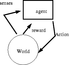
The world receives the action of the agent. Under certain circumstances, the agent receives a reward. The agent adjusts its action to maximize the reward.

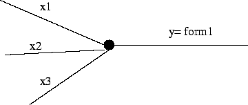
This is the simplest non-trivial model of a neuron.
If we have several trials (Indexed by ![]() which could be time, but
almost never is in these cases.), then there are vectors
which could be time, but
almost never is in these cases.), then there are vectors
![]() and outputs
and outputs ![]() , as well as desired outputs
, as well as desired outputs ![]() .
.
|
Our Goal:
Find an incremental way of finding the optimal

|
We let
![]() change by
change by
![]() , where
, where ![]() is precisely described as
``small''.
is precisely described as
``small''.
The
![]() coordinate of
coordinate of
![]() for the
for the
![]() trial is computed via:
trial is computed via:
So that the update rule is given by (1)
Whenever we analyze one of these methods, we are concerned with the following questions:
When we slect ![]() , we have to keep in mind that choosing an
, we have to keep in mind that choosing an ![]() that is too small may cause slow convergence, while choosing an
that is too small may cause slow convergence, while choosing an ![]() too large may cause us to skip over the minimum point (see figure
1.1.3)
too large may cause us to skip over the minimum point (see figure
1.1.3)
We want to choose ![]() so that the successive approximations
converge to some position in weight space.
so that the successive approximations
converge to some position in weight space.
If we teach the neuron with several trials, the total error is
![]() . This is the average of the errors.
. This is the average of the errors.
| It is important to include several trials, since, if |
Widrow-Hopf LMS was first used in adaptive radar beam forming programs in the late 50's and early 60's.
The perceptron problem includes the following:

Given a putative
![]() , we get that
, we get that
![]() whenever
whenever
![]() .
.
![]() is a line in
is a line in
![]() space with dimension
space with dimension ![]() and with normal
and with normal
![]() . One side of this hyperplane consists of all
. One side of this hyperplane consists of all
![]() that will yield an on position, and the other side consists of all
that will yield an on position, and the other side consists of all
![]() values that will yield an off position.
values that will yield an off position.
Since our trials tell us what
![]() values
actually yield on and off, choosing the
values
actually yield on and off, choosing the
![]() and
and
![]() is a matter of choosing a plane that puts the on and off dots
on the correct sides (see figure 1.2.2).
is a matter of choosing a plane that puts the on and off dots
on the correct sides (see figure 1.2.2).
For the sake of simplicity, let
![]() for a moment. It is easy
to take care of the
for a moment. It is easy
to take care of the ![]() afterards.
afterards.
We want change ![]() thus:
thus:
|
Let
Let |
We would like to guarantee that
![]() , so that
, so that
![]() .
.
This means that:
![]() .
.
So that:
![]()
If we say
![]() .
.
Where ![]() is just barely large enough to force the
is just barely large enough to force the ![]() to
change sign. (Remember that the
to
change sign. (Remember that the ![]() was set to the largest possible
value that would not change the sign.)
was set to the largest possible
value that would not change the sign.)
We still want to know :
we here implement the perceptron learning problem as a batch solution:
Given trials indexed (again) by ![]() , we have
, we have
![]() and
and ![]() . and
. and
![]() . For some
. For some ![]() ,
,
![]() , and for some,
, and for some,
![]() . In order for each of the trials to match
the desired value, we need
. In order for each of the trials to match
the desired value, we need
![]() for
all
for
all ![]() . This is a linear programming problem. Every
. This is a linear programming problem. Every ![]() defines a
half space in
defines a
half space in
![]() - coordinates defined by
- coordinates defined by
![]() , and
the possible
, and
the possible
![]() 's must lie in the intersection of all these
spaces.
's must lie in the intersection of all these
spaces.
This document was generated using the LaTeX2HTML translator Version 99.1 release (March 30, 1999)
Copyright © 1993, 1994, 1995, 1996,
Nikos Drakos,
Computer Based Learning Unit, University of Leeds.
Copyright © 1997, 1998, 1999,
Ross Moore,
Mathematics Department, Macquarie University, Sydney.
The command line arguments were:
latex2html -split 1 -white 8_28.tex
The translation was initiated by Ben Jones on 2000-08-30